Sky Charts
Configuration details
Configuring the appearance of objects
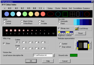
This panel allows you to change the appearance of
the stars and nebulae.
The first section gives you the option of changing
the colors of the stars and nebulae according to
their B-V color index, the background color and the
coordinate grids. These colors are used for line
drawing and color printing.
Click on the corresponding element to change its
color.
The section "Colors" gives you the option of choosing the appearance, in color, black and white, or red. The selection "Invisible" displays labels without displaying the objects.
The sky color can be fixed as defined in the first section or be set to automatically change to reflect the actual sky luminosity. You can also change the sky color for the different twilight phases by clicking in the blue rectangles after "Automatic" has been selected.
The next selection lets you adjust the size of the
stars according to their magnitude. Use the buttons
brightness +/- and contrast +/- to alter the absolute
or relative size of the stars. The "Reset" button
returns the contrast and brightness to their default
values.
The box "Bitmap stars" controls the display mode for
the stars. Once selected you can also change the
bitmap file used to draw the stars. The file
MediumLightColor resets the image to the default
value. Some of these files are available with the
program but you can also create your own.
The file characteristics are:
Each star must be in a square area containing an odd
number of pixel (i.e. 21x21), the star is centered in
this area.
There are 11 areas for each line corresponding to
the different magnitudes.
There are 7 lines, one for each B-V color index
range.
Next, select "Show" if you want to display the Milky Way and the desired isophote line or hash.
The nebulae drawing can be a color symbol as defined in the first section or a gray surface. If you select the gray surface you can adjust the gray level used to represent the various surface brightnesses of the objects.
The last line lets you choose the file containing the
description of your local horizon.
Each line of the file must contain two values: the
azimuth (integer value) and the corresponding
altitude.
It is not necessary to indicate a value for each
azimuth as intermediate values are interpolated. But
the line must be in increasing order of azimuth from
0 to 359. The file horizon_Geneve.txt is an example
of my local horizon in Geneva. If you create your own
local horizon file, I suggest you name the file
according to your place name.
Selecting "Invisible" removes all objects below the
horizon of the chart. "Ground Color" permits you to
choose the color of the chart below the horizon.
Labelling objects
It is possible to assign a label to the type of object that has been selected:
If the option "Display" is checked, then a label is displayed for all selected objects.
The option "Options" lets you choose the information you want to display (name, magnitude, coordinates), where the information is displayed (left or right), the label text color and size, and the type of object that is to be displayed. The magnitude limit prevents displaying a label for fainter objects.
The option "Short Name" will use the shortest posible name for the label, i.e. a greek letter for the bright stars.
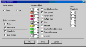
The choice "Individual Selection" means that only
the selected objects will be given a permanent label
until you remove them with the option "Clear
Selection". It is also possible to remove the last
entered label.
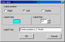
Free Label
The "Add Label" option of the chart popup menu (right
click on chart) lets you enter text anywhere in the
chart. Select the label position relative to the
cursor position, the color and size. Then type the
text you want.
Date and Time
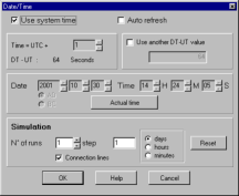
Define the date and time used to calculate the
position of the planets, comets, asteroids as well as
the azimuth position and the proper motion.
It is possible to use the system date and time or
you can enter any valid date and time between year
-20000 and +20000. The planet positions are only
calculated for a date from -3000 to +3000. Beware
with the negative year: 1BC is the year 0 and 2BC is
the year -1.
If the option "Auto Refresh" has been selected, then
the time is updated every minute. Otherwise the time
used throughout the session will be the time the
program was launched unless manually refreshed with
the button "Actual time".
The time zone has to be given relative to UTC. Enter
the difference in hours to obtain your local time.
This number is positive if you are located east of
Greenwich and negative if you are located west of
it.
The difference between the dynamic time used by the
program and the standard time is automatically
calculated. If you want to use another value just
check the box and modify the value.
Simulation:
It is possible to calculate an object's position for
several dates.
Give the number of dates you would like, the
interval between them and if you want to connect the
different position by a line. See also animation.
Observatory
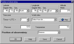
Define the location of the observation site to be
used when calculating the parallax and the azimuth
position.
Enter the latitude, the longitude, the altitude (in
metres) and the time zone of your observatory.
Enter also the pressure (in millibar) and the
temperature (in Celsius degree) to be use to
calculate the atmospheric refraction.
You can assign a name to a location. Press "Save" to
keep it for next session. It will appear in the list
of the available locations.
As a first approximation you can also use the list
of the major world cities.
If you don't know your observatory coordinates click
"Map" and select your location on the map using the
mouse.
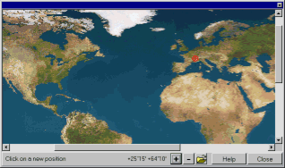
It is possible to zoom or to replace this map by
another of your choice, the only restriction is it
must use the same projection.
Projection types
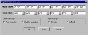
This panel lets you choose the projection you want
to use when displaying a chart according to the
selected field width, the chart orientation and the
azimuth origin.
- Polar projection is the conventionnal celestial atlas representation with North Pole at the top. Coordinates are always ICRS (J2000) independently of the date.
- Zenithal projection represents the actual sky from a given location at a given time with the zenith at the top. Coordinates are those corresponding to the actual date. It is possible to choose the azimuth origin from North or from South.
The available projections are:
- ARC: Arc length. It is the default projection up to 180°. It corresponds to the projection of a Schmidt camera.
- TAN: Tangent. Corresponds to the projection of a picture obtained with a telescope or a photographic lens.
- SIN: Sine. Used to display images in radio-astronomy.
- CAR: Cartesian. The default projection between 180° and 360°. It is of no great interest apart from the fact that it can display very large field of views.
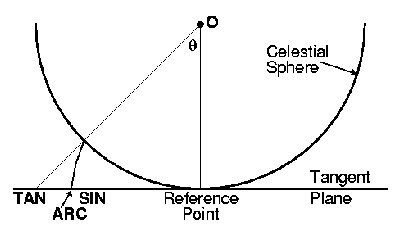
by E. Griessen, AIPS memo 27
The selected projection described up to here can be
modified according to the header of the file in FITS
format containing WCS when you load such an
image.
Displaying images
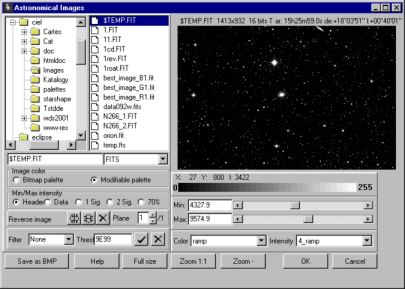
This panel lets you select the image that will be
displayed with the chart.
The image is loaded in a preview window. You can
modify the display tresholds (min and max), the color
palette (composite colors LUT and intensity tables
ITT) and zoom a portion of the image using the
mouse.
It is also possible to display the image in its
original dimension and then zoom it by using the +
and - keys.
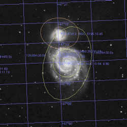
For FITS format files, which contain the coordinates RA, DE or GLAT, GLON (i.e. the images provided from DSS-ESO or IRAS) the program uses the coordinates and the projection from the header of the FITS format to automatically position the image in relation to the current chart. Please note that it is only possible to zoom a section of the image from the preview window and not on the main screen, otherwise the automatic positioning does not work. For other image formats it is necessary to place the image on the chart manually. You can of course use the function "Online Resources "to download an image directly from the Internet.
It is possible to derive the initial thresholds from
the information contained in the file header, from
the lowest and highest values or from the average
plus one or two standard deviation values.
If the image file contains more than one plane
(NAXIS3 > 1) you can select between them with the
option "Plane".
If the sequence of the pixels is not standard you
can mirror the image with the option "Reverse
Image".
You may also apply a convolution filter to the
image. Only pixels with a value below the treshold
are filtered.
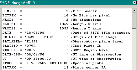
The right mouse button clicked on a file name displays the header of the file in the format FITS or PIC.
For bitmap formats check the option "Bitmap Palette" from the selection box "Image Color". In this case all the other functions are disabled. Otherwise and if the image is a 24 bit format, the program generates a gray level from the average of all the RGB planes (plane=0) or each color independently (plane=1,2,3). In both cases the image can be modified as FITS or PIC format files.
You can save the current image in a file in BMP format and reuse it later with the same appearance.
The following formats are supported:
FITS integer 8,16,32 bits, real 32,64
bits *.fit *.fts *.fits
PIC (MIPS) integer 16 bits
*.pic
Bitmap 8,24 bits *.bmp
*.dib
JPEG *.jpg *.jpeg (not
progressive)
GIF *.gif (not
progressive)
TGA *.tga
RLE *.rle
PCX *.pcx
The OK button loads the image into the current chart.
Note regarding the coordinates of the FITS
files:
Unfortunately there is not a unique and standardized
way of describing the WCS in a FITS file. This
program supports the three most common methods :
CROTA2, CDi_j, PCiiijjj.
It has been tested with many files obtained from
different sources. It is however impossible to
guarantee that a particular file has not implemented
a variation of this format. In this case an error
would certainly arise. If you are not certain of the
format of an image please consult the comments in the
header of the file.
Bulk calculation of asteroids
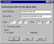
This function computes the position of all asteroids
for a given date.
Please enter the complete path to the file
"astorb.dat" and of the resulting file, the date and
time of the observation and if the position has to
consider the topocentric parallax.
It is advisable to keep the original values for the
names of the files.
The update of astorb.dat is available using the "Online Resources" option.
Select if you want to display the position of the
asteroids on the chart according to the magnitude or
to the size of a symbol. To modify this choice later
or to suppress the display of the asteroids, use the
external catalog
function at the line Astorb.
On a Pentium 166 it takes 40 seconds to calculate
the position of 40,000 asteroids.
Warning !
The original astorb.dat file is in UNIX format
(end-of-line = LF). You must convert it to the DOS
format (end-of-line = CR+LF) before you can use it
with "Sky Charts". This done automaticaly if you use
the "Online Resources" option to load the file.
Online Resources
This menu takes you directly to the Internet
resources.
You must be connected to the Internet before you can
use this function.
If you want more information on the home pages
themselves, just click on the information URL.
The following resources are available:
Images corresponding to displayed chart:
- SkyView : Images in all wave lengths
- ESO Skycat Digitized Sky Survey : Palomar atlas for the whole sky. The image dimension is limited to 1600 square minutes. The size of the corresponding file is 2.5 KB multiplied by the square size in minutes.
- ESO Skycat Digitized Sky Survey 2: The same survey but with a 15 micron scan rather than 25 micron. The pixel resolution is 1 arcsec instead of 1.7 arcsec. The files are three times bigger.
Extraction of large star catalogs:
The data requested from these catalogs corresponding to the current chart is stored in a temporary file and automatically defined as catalog according to the magnitude, the disabling is done in this panel.
HST Guide Star Catalog (20,000,000 stars)
- CDS VizieR: Stars up to the magnitude 15. The field is limited to 5 degrees or 5000 stars.
- ESO Skycat: Stars
up to magnitude 15. The field is limited to 2 degrees
or 1000 stars.
USNO-A (526,000,000 stars)
- CDS Vizier: USNO-A2.0 Stars up to magnitude 20. The field is limited to 2 degrees or 5000 stars.
- ESO Skycat: USNO-A1.0 Stars up to magnitude 20. The field is limited to 2 degrees or 5000 stars.
GSC 2.2 (455,851,237 stars)
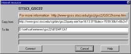
- STSCI GSC 2.2: Stars up to magnitude 18.5. The field is limited to 1 degree or 5000 stars.
Comets and asteroids
Data from CBAT/MPC
:
- Update of the currently visible comets. If a file CAT\PLANET\COMETES.OLD exists, then this file is appended to the transferred file. This feature lets you keep old elements originating from previous observations.
- Update of the bright asteroid list at opposition during the current year.
- Update the asteroid list from ASTORB data base to file CAT\PLANET\ASTORB.DAT. This list contains recent elements for more than 150,000 asteroids. Beware that this file is growing rapidly and is now very large to download.
You can carefully modify some default options in the
file EXTRES.INI. If you want to use a proxy server
follow these instructions:
Remove the semicolon for the three lines at the
beginning of the file concerning the proxy. Change
the IP address and the port number for your server.
The file must look like this:
[proxy]
proxy=192.168.0.1
proxyport=8080
Beware that this file is replaced by a new version
or an upgrade.
HEASARC SkyView
This panel gives you the ability to directly obtain a
sky image corresponding to the current chart.
You must be connected to the Internet before you can
use this function.
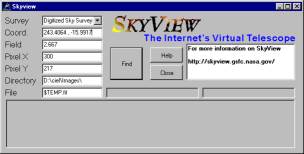
If you need more information on SkyView or if you
wish to obtain the description of all available
catalogs as well as the dimension limits, please
consult http://skyview.gsfc.nasa.gov
Do not modify the default value of "Coord" and
"Field" if you want an image for the current
chart.
Otherwise you can give an object name in the field
"Coord", which will be resolved by SIMBAD.
The size of certain catalogs is limited (i.e. 4°
in the case of the DSS).
Pixel X and Pixel Y represent the number of pixels of
the image. If these two fields are empty, then the
resolution of the catalog will be used.
Warning: keep an eye on the size of the file you are
going to transfer!
If you plan to keep the file for later use, give it a name in the corresponding field but do not modify the extension ".fit".
Estimation of the file size:
The data has a depth of 32 bits and the header is
negligible.
The size in bytes is: pixelx * pixely * 4 giving 360
KB for an image of 300x300.