Field Rotation, Polar Alignment, and Declination Drift
Calculations, Formulas and Relation to Astrophotography

Part I: Altitude-azimuth mounts

When using an alt-azimuth mount to look at things in the sky, even with a mount that is capable of tracking the stars (such as the Meade LX200 series), images will appear to rotate within the eyepiece field. This phenomenon is known as field rotation.

It is easy to understand how this arises by considering a specific example. Imagine we are at the equator looking at a pair of stars very near the north (or south) pole - i.e. very close to the horizon - such that the two stars happen to have the same Right Ascension (RA). Let's draw a line through them; in fact this line will coincide with their RA line. As the stars rise above the horizon, this line will be almost parallel to the horizon. When the stars pass through the meridian, this line will be vertical with the horizon; in fact it will coincide with the meridian. Finally as the stars set the line will once again be parallel to the horizon again. Now imagine that we are looking at the stars with a telescope and - for our current purposes - an eyepiece with a rectangular field of view such that one side of the rectangle is parallel to the horizon. The manner by which alt-azimuth mounts work ensure that this side of the rectangle would always remain parallel to the horizon (remember lines of constant altitude are parallel to the horizon). However, I just mentioned that the line drawn through our pair of stars will appear to rotate with respect to the horizon, which means when viewed through our rectangular telescope field of view they will certainly rotate as well. With a little extra thought, it is easy to see that this field rotation is really independent of the shape of the eyepiece field of view.

Field rotation isn't really an issue for visual observing, but when trying to perform astrophotography, field rotation means that there is a certain maximum exposure time you can use for an alt-azimuth mount driven photographic instrument before your stars become recorded as arcs.

This page describes my attempts to calculate the exact magnitude of field rotation as a function of the astronomer's latitude. Following which I will also try to derive an expression for the maximum exposure time allowed before noticeable image smearing occurs, specifically in the context of high power planetary photography. I shall assume the reader understands multivariable and vector calculus, as well as some very elementary ideas from differential geometry. Please do let me know if you spot any computational or other mathematical errors.

For convenience let's imagine our stars are all stuck on a unit sphere and we as observers are mathematical points right at the center of the sphere. For a given object in the sky (i.e. on the unit sphere), we can specify its coordinates by using a cartesian system (x, y, z).  This can also be related to its right ascension and declination, or to its altitude and azimuth. Let's spend some time setting up these two different sets of coordinates on the unit sphere. (You may wonder why we need two sets of coordinates - please read on to find out.)

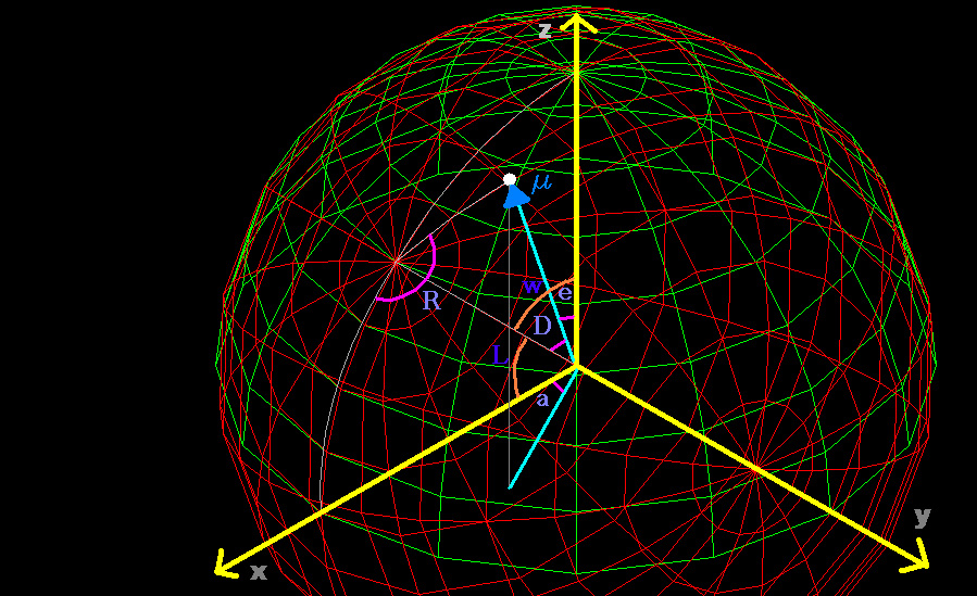
Let's start with the altitude-azimuth coordinates. If we let the x-y plane represent the apparent plane (horizon) we observe from, the z axis would point to the zenith. Given a star on the sphere, let the angle subtended by the z axis and the radial line joining the star and our sphere center (also the center of our x-y-z axes) be e. Project the star perpendicularly upon the x-y plane and draw a line from the projected point to (0,0,0). Denote the angle subtended by this line and the x axis as a. These {e, a} coordinates are very similar to altitude and azimuth coordinates, except that I've chosen them this way to help make calculations easier.

We thus have, the coordinates of a given point on the sphere µ[e, a] = (x, y, z) = (sin[e] cos[a], sin[e] sin[a], cos[e]).

Let's set up the right ascension-declination-like coordinates. Because we won't really be interested in the exact right ascension of the objects in question, I propose to use the following system to make calculations easier. Imagine that in place of the above {e, a} coordinates, I change their names to {R, D} instead. Then I rotate the whole sphere about the y axis by an angle w (without rotating the axes themselves - otherwise we're back to the same situation). Notice this set of new rotated {R, D} coordinates is similar to an RA-Dec system for a latitude of (90 degrees - w degrees).  Mathematically this means we replace the above {e, a} with {R, D} and multiply the above vector by a rotation matrix.



After some trigonometry and linear algebra we have µ[R, D] = (x, y, z) = (cos[R] cos[w] sin[D] + cos[D] sin[w], sin[D] sin[R], cos[D] cos[w] - cos[R] sin[D] sin[w]).

But I'd ultimately want my formulas in terms of R, D so it'd be more convenient to shift coordinates such that the sines and cosines of w appears with the e and a. But since rotation matrices are easy to invert we obtain immediately

µ[R, D] = (x, y, z) = (sin[R] cos[D], sin[R] sin[D], cos[R]) = µ[e, a] = (x, y, z) = (cos[e] cos[w] sin[a] - cos[a] sin[w], sin[a] sin[e], cos[a] cos[w] + cos[e] sin[a] sin[w]).

An alt-azimuth mount that tracks the stars is one that moves in such a way that a scope mounted on it will point always at the same constant-declination line in the sky (i.e. on the unit sphere). Imagine that we can see two sets of finely spaced grids superimposed on our sky as we look through a telescope mounted on such a mount: one set is that of the altitude-azimuth, and the other the RA-Dec. Because ours is a alt-azimuth mount, the altitude-azimuth grid will not appear to rotate as we follow the stars, but the RA-Dec lines would, for the reasons already discussed earlier; whereas the orientation of objects in the sky (e.g. the direction of the line drawn through our hypothetical pair of stars) stay fixed with respect to the RA-Dec grid (e.g. the line through the 2 stars stay on top of a particular constant-RA line). This makes us realize that field rotation at a given point in the sky is really the rate of change of the angle formed by either the RA line or the Dec line with the azimuth or altitude line passing through it as we move along in RA while tracking the stars.  In more technical language, we need to obtain two frames at every point on the sphere: one with unit vectors parallel to the RA and Dec lines passing through the given point, and the other with unit vectors parallel to the azimuth and altitude lines passing through the same. As the mount tracks, it moves in RA; but because it is an alt-azimuth mount, it "remains" set in the latter frame field, while the former RA-Dec frame field rotates with respect to the latter.

Since we are interested in angles only, we need only to obtain one vector for each frame.

For the RA-Dec frame, I got the vector pointing parallel to the constant Dec line by differentiating µ[R, D] with respect to R, to obtain dµ/dR = (-Sin[D] Sin[R], Cos[R] Sin[D], 0). By taking dot product with itself, we see the length of the vector is (Sin[D])^2, and so the unit vector is r_hat = (1/Sin[D) (-Sin[D] Sin[R], Cos[R] Sin[D], 0).

For the altitude-azimuth frame, I got the vector pointing parallel to the constant altitude line by differentiating µ[R, D] with respect to e, to obtain dµ/de = (Cos[D] Cos[R] dD/de - dR/de Sin[D] Sin[R], Cos[R] dR/de Sin[D] + Cos[D] dD/de Sin[R], dD/de Sin[D]). Taking dot products with itself we see its length is (dD/de^2 + dR/de^2 Sin^2[D])^0.5. The corresponding unit vector is thus E_hat = (dD/de^2 + dR/de^2 Sin^2[D])^0.5 (Cos[D] Cos[R] dD/de - dR/de Sin[D] Sin[R], Cos[R] dR/de Sin[D] + Cos[D] dD/de Sin[R], dD/de Sin[D]).

We need to figure out what dD/de and dR/de are. To do that we refer to the fact that µ[R, D] = µ[e, a] since they really are the same vector. Look at the z component of the matrix equation: cos[e] = cos[D] cos[w] - cos[R] sin[D] sin[w]. By differentiating both sides with respect to R, with respect to D, using the relation sin^2 + cos^2 = 1, and using the fact that dx/dy = 1/(dy/dx), we can then obtain dR/de and dD/de.


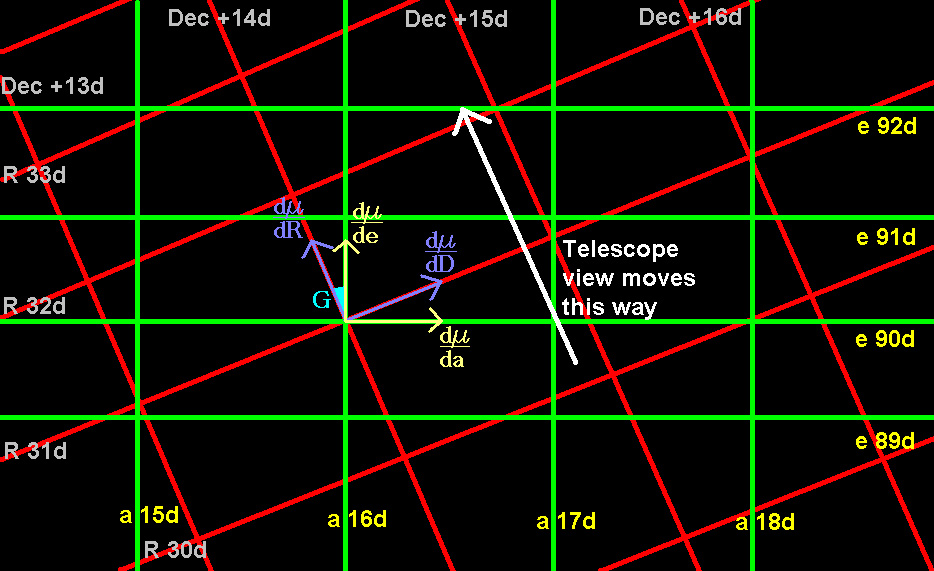
A "zoomed-in" view of the two sets of coordinate systems around a given point on the celestial sphere. The two frames used in our calculations are shown with the un-normalized vectors. It is difficult to draw curved lines, so I drew straight lines - in reality, coordinate lines are curved. With some imagination, one can see how field rotation occurs: the alt-azimuth mounted telescope delivers a view in which the {e, a} frame (indicated by the dµ/de and dµ/da vectors) does not rotate; and at the same tine the orientation of the celestial objects stay fixed with respect to the RA-Dec grid (and hence with respect to the {R, D} frame, indicated by the dµ/dR and dµ/dD vectors). Now the telescope, if tracking, moves along in RA (or, in our system of variables, simply R). Because the coordinate lines are generally curved, the angle G between the frame vectors dµ/dR and dµ/de will change as R changes, giving rise to field rotation. This way of thinking about field rotation also forms the basis of our calculations. (Note that I have made no effort to make the R, Dec, e, and a scales consistent, because they are merely there for illustrative purposes. For instance, {e, a} = {90d, 16d} is most certainly not the same point as {R, Dec} = {31d, +14d}.)

From vector analysis we have r_hat . E_hat = || r_hat || || E_hat || cos[G] = cos[G], where G is the angle between the two unit vectors from the RA-Dec and alt-azimuth frame fields. We want to find out what the rate of change of this angle G is when our mount tracks in RA, so we now differentiate both sides with respect to R. (d/dR) (r_hat . E_hat) = -Sin [G] dG/dR. By using the relation sin^2 + cos^2 = 1 again, we therefore get an expression for dG/dR. But we already have the expressions for r_hat and E_hat, so all I needed to do was to plug them into Mathematica. Furthermore, what we really want is dG/dt, the rate of rotation with time, so we do dG/dt = dG/dR x dR/dt, where dR/dt is simply the rate of rotation of the earth, which is 2 pi (i.e. 360 degrees) divided by one sidereal day (23.93446965 x 60 x 60 seconds).


dG/dt =

 

where the units is in radians per second, R is our pseudo-RA coordinate, D is our pseudo-Dec coordinate, and L is our observer's latitude. To convert D to the usual declination d, note that for D = 0 degrees, d = +90 degrees; D = +90 degrees, d = 0; D = +180 degrees, d = -90 degrees.)

One of the practical applications of the above formula is the following. I have been thinking of discarding my heavy equatorial mount and small telescope and replacing it with a large Dob with a driven alt-azimuth mount. However, I want to use it to do high resolution photography of the planets. The question is how long an exposure can I make without having my image smeared and blurred by field rotation?

To consider this let's suppose the radius of our planet is sigma in arc seconds. We shall also assume that our planet is placed right at the center of our field of view; one should keep this in mind when doing planetary photography. After a time tau seconds, the planet as seen in my Dob would have rotated by roughly dG/dt x tau radians; which means a given point on the circumference would have moved by an angular distance of dG/dt x tau x sigma. (The exact expression can be obtained in at least two ways. One would require replacing R with an appropriate time dependent expression - e.g. R = 23.93446965 x 60 x 60 t - in the above formula, and then integrating it with respect to t over the appropriate limits. The other would be to replace R, with the time dependent expression, in the just-worked-out r_hat . E_hat = Cos[G] and then plug in the appropriate starting and ending times to obtain two separate sets of equations, take the inverse cosines of both sides, and subtract.) Because the circumference of the planet would be most smeared, it suffices to ensure that a given point on the circumference would not appear smeared after a given time tau. Now to have a smeared image the angular distance traveled by a given point must be greater than roughly half the smallest angular distance that can be resolved by the telescope. The latter (in radians) is given by a well known formula: 1.22 x lambda / diameter of scope, where lambda is the wavelength of light - since we are looking for the maximum allowed time, we may as well plug in the shortest wavelength (i.e. the most sensitive) of visible light: 4 x 10^-7 m.

This means dG/dt x tau x sigma < (1/2) (1.22 x 4 x 10^-7) / Diameter, which leads to the maximum allowed time tau is

 

where R, D and L are as before, Gamma is the diameter of the telescope in inches, and Sigma is the radius of the planet in arc seconds.

As a concrete example, for the August 2003 opposition of Mars, the red planet would have a radius (sigma) of roughly 12'' and declination of approximately +14 degrees (D = 90 degrees - 14 degrees). If I'm observing from Singapore (latitude of 1 degree, which I will round off to zero) with a 10 inch Dob, the following is the plot of maximum allowed exposure time over the entire movement across the sky (i.e. over the range of R from 0 to 2 x pi).

  

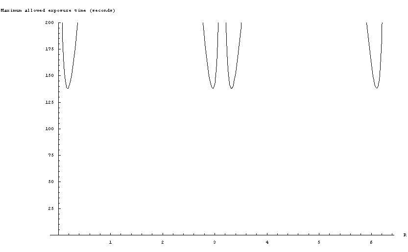
As you can see the minimum is greater than 135 seconds, or 1 min 15 s. This is very sufficient for planetary photography since exposures rarely exceed several seconds (not advisable anyway, due to turbulence). Even if the planet is placed off center by a distance of say 10 radii, we would still have a minimum of 13 seconds, adequate time for photography with webcams and high speed films. However, this illustrates why alt-azimuth mounts without field rotators are impractical for deepsky astrophotography since the relevant radius (sigma) in that case much greater, and hence the maximum allowed time is much shorter, while the exposure time needed is usually at least tens of minutes.

Part II: Equatorial Mounts

A little thought reveals that we can use our results above to solve a related problem in deepsky astrophotography for equatorial mount users.

It is impossible to achieve perfect polar alignment. This error in polar alignment leads to field rotation problems similar to the one described above. The natural question is then, how close to the true pole must one align his/her equatorial mount axis in order not to suffer from field rotation effects in a guided photograph for a given desired length of exposure?

Earlier, we used the {e, a} coordinate system to represent movement by the alt-azimuth mount - images viewed through a scope placed on such a driven mount would not rotate with respect to the local {e, a} grid. Now we can use the same {e, a} grid to represent movement by an equatorial mount, except the grid would now have to be rotated such that the e = 0 point (i.e. the mount's north pole) would be located close to the D = 0 point (i.e. the north celestial pole), where the angular distance between the e = 0 point and D = 0 point as measured from the center of the sphere (0, 0, 0) would then be the error in polar alignment. But this is simply equivalent to the above problem if we observe that the variable w = (90 - L) degrees we used above is exactly the polar alignment error we are currently pursuing.

By replacing L with (90 - w) degrees, I went on to find out, for a given exposure time, which areas of the sky would not suffer from field rotation effects when photographed. By assuming that I use a perfect autoguider guiding on a star right at the center of my photograph, I made plots for my 5" refractor (770mm focal length), which gives approximately a 2.68 degrees wide field on the 36mm side of the 35mm film format.

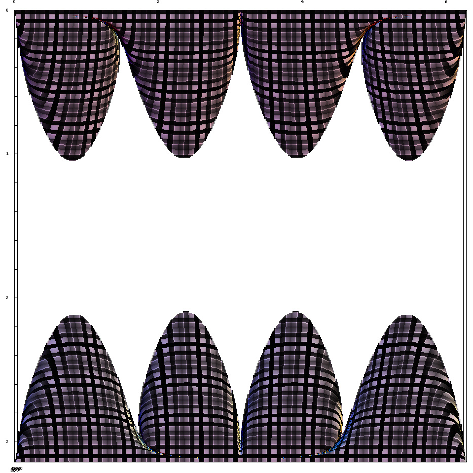
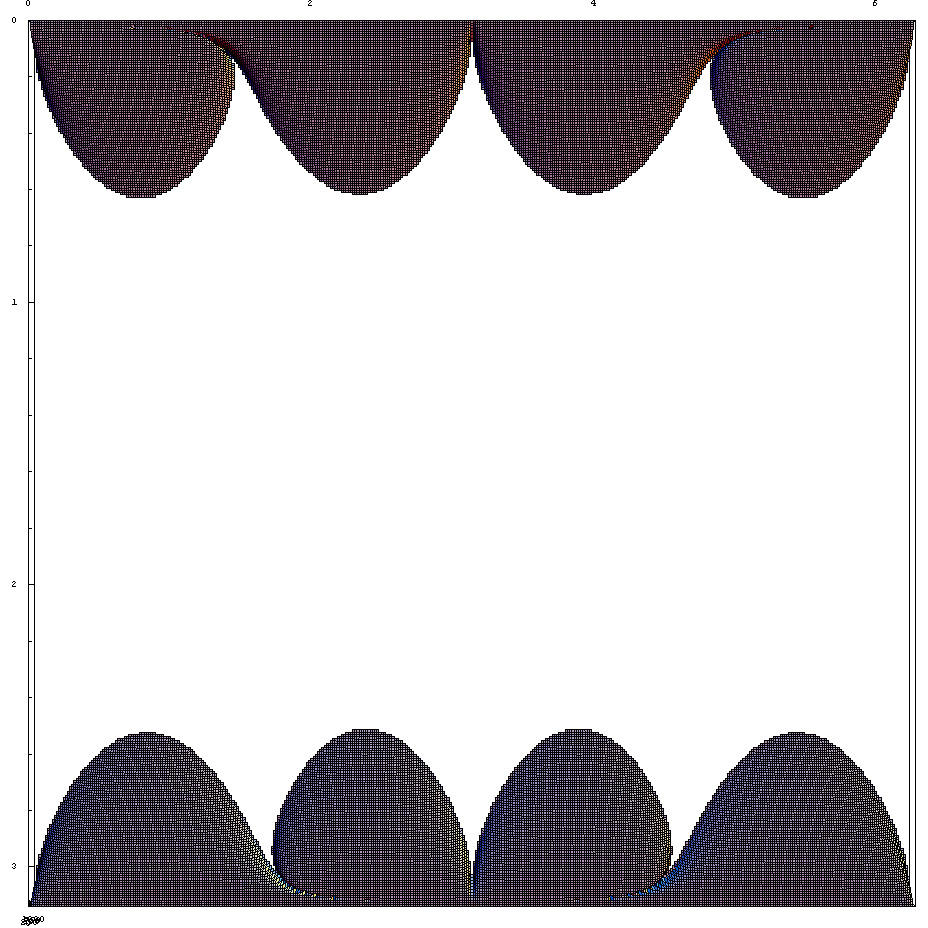
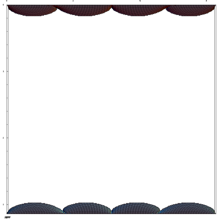
First I looked at the case for a 20 minutes exposure.

Polar alignment Error: 1.5 degrees (Vertical Axis: D, Horizontal Axis: R)



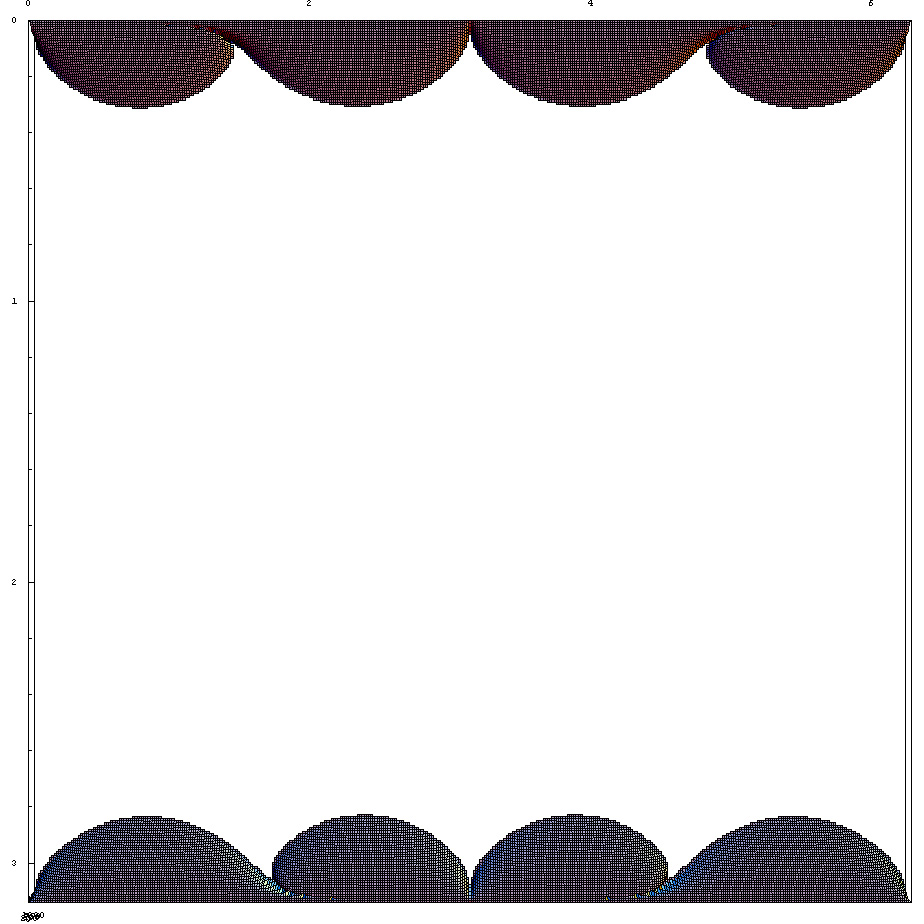
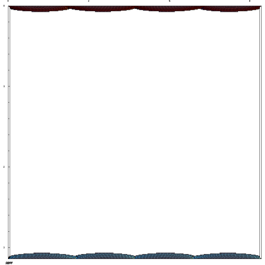
Polar alignment Error: 1 degree (Vertical Axis: D, Horizontal Axis: R)



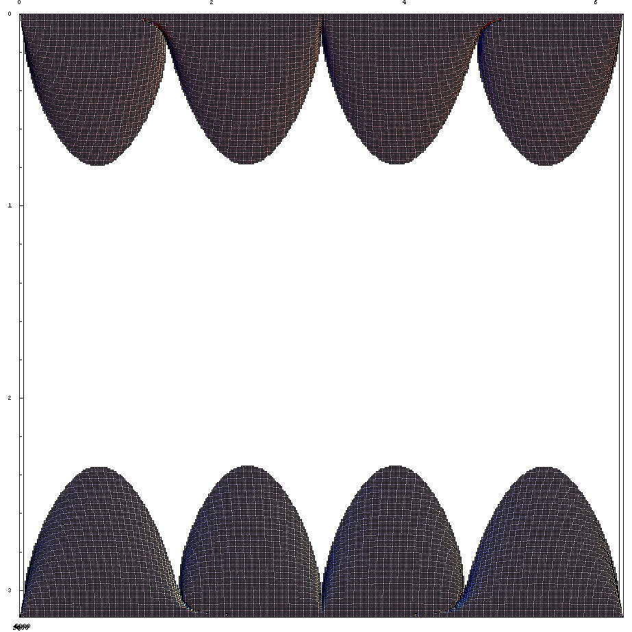
Polar alignment Error: 0.5 degree (Vertical Axis: D, Horizontal Axis: R)



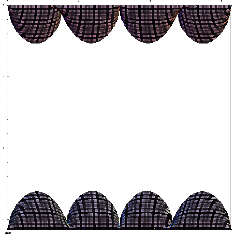
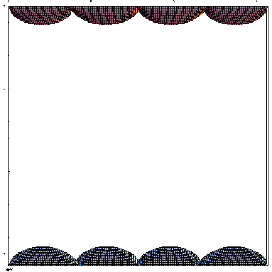
Polar alignment Error: 0.15 degree (Vertical Axis: D, Horizontal Axis: R)


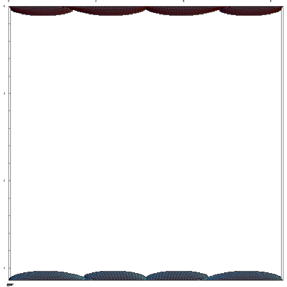
These plots show the regions of sky that can be photographed with my 5" refractor without suffering from field rotation effects over a duration of 20 minutes. The vertical axis is our pseudo-Dec coordinate (in radians), which means the top of the plot is the celestial north pole, the middle are the mid-latitudes, and the bottom is the south pole. The horizontal axis is our pseudo-RA coordinate (in radians), which means if you look at the plot from left to right you are looking at the sky from the eastern hemisphere meridian to the western hemisphere meridian and then back to the eastern hemisphere meridian (actually east and west is dependent on your definition, but I hope one gets the idea - if not look at my first diagram on this page). The white areas are the regions in the sky that can be photographed without suffering from field rotation effects, whereas the colored regions cannot. (These diagrams are really 3D plots of (x, y, z) = (R, D, tau). We are viewing them 'face-on,' from the 'bottom,' in order to achieve this seemingly 2D perspective, ignoring the tau axis.)

We observe immediately two things. The first is that the polar regions suffer the most from field rotation effects; or to put it in another way, if you wish to photograph the polar regions, you'd need to polar align your mount much more accurately than you'd need to for photographing the equatorial regions. The second is that polar alignment for deepsky astrophotography really needs to be accurate - we see that even with an error of only 1 degree and a relatively short exposure of 20 minutes, roughly 35 degrees of sky around each pole cannot be photographed successfully.

Here are two more examples for the same telescope. The first is for a 1 hour exposure.

Polar alignment Error: 0.5 degrees (Vertical Axis: D, Horizontal Axis: R)



Polar alignment Error: 0.15 degrees (Vertical Axis: D, Horizontal Axis: R)



Polar alignment Error: 0.05 degrees (Vertical Axis: D, Horizontal Axis: R)



The second example is for a 2 hour exposure. Notice how accurate polar alignment needs to be for this case - even a 0.5 degree error in polar alignment leaves much of the sky unsuitable for photography.

Polar alignment Error: 0.5 degrees (Vertical Axis: D, Horizontal Axis: R)



Polar alignment Error: 0.15 degrees (Vertical Axis: D, Horizontal Axis: R)




We can summarize the results as follows:

1) The larger the aperture of your photographic instrument (the larger the Gamma), the higher its resolution, and hence the more sensitive your photograph will be to mis-polar alignment.

2) The wider the field of view of your photographic instrument - and hence the larger the radius of rotation (sigma) - the more susceptible your photograph is to mis-polar alignment errors.

3) To minimize field rotation problems, always try to guide near the center of your photograph. The key is one needs to minimize the angular distance between the guide star and the farthest point from it in your photograph.

4) Be especially careful in polar alignment when photographing near the poles.

Part III: Declination Drift

We can solve yet another problem quite easily, with the work already done above. This is the issue of declination drift. When performing polar alignment, astrophotographers usually use what is called the drift alignment method for polar alignment. After roughly aligning the polar axis of her/his mount to the north, the astrophotographer usually proceeds to point her/his telescope to a star low in the east (or west), center it on usually a crosshair and watch which way it drifts in declination as the mount tracks the star with its motor drive on. There is a standard procedure to determine the corresponding adjustments needed. (With a little extra effort, one can also derive the procedures from the current discussion.) Next the astronomer looks at a star on the meridian and performs similar observations and adjustments. The question that then naturally arises is, how much declination drift within a given time interval is acceptable if one desires to obtain a non-field rotated photograph - i.e. the field rotation effects do not smear the stars sufficiently to be noticeable?

First I recall a result I obtained above, but did not display. I calculated the cosine of the angle G (Cos[G]), which in the present case is really the angle between the instantaneous direction of movement of the telescope's center of view and that of the star at the center of its view at a given moment. Now the earth and the mount rotate at a rate of u = (2 Pi) / (23.93446965 x 60 x 60) per second. That means in a small time interval, the apparent movements of the center of the telescope's view and the star would appear to each trace out a line, which when taken together forms a small wedge. This small wedge can be taken as a flat triangle (in Euclidean space) as a first approximation - even though they actually sweep out arcs on the unit sphere defined above. Then, assuming the angle of the wedge is small, we can further assume that the declination drift can also be approximated by the circular arc subtended by the two lines forming the wedge, even though to be precise we'd need to resolve it into perpendicular (aka declination drift) and parallel (aka RA drift) components and also take into account the curvature of our unit sphere.

Let t be the time that has passed since our astronomer began watching the star. Both the telescope's center of view and the star would have swept out an angular distance of (u t). That means the distance between the ends of the two lines is, roughly G x (u t). That is our desired declination drift, in radians:



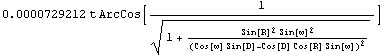
For the same formula in arc seconds - a more useful unit for practical declination drift purposes, we divide by 2 Pi and multiply by (360 x 60 x 60) arc seconds:

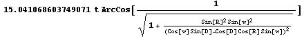             [Dt]

where t is the total amount of time in seconds star has been allowed to drift from the center of view, w is the angular distance the true celestial pole is displaced from the mount's polar axis (aka polar misalignment), D and R are the pseudo-RA and Dec coordinates defined above in Part I.

Suppose we have figured out - say from the considerations described in Part II above - that we need to get the mount's polar axis within w radians (or degrees - whichever you wish to plug in) of the true pole. And suppose we're only patient enough to watch the star drift for t seconds (e.g. a common time used is 300 seconds, or 5 minutes). Then how much can the star drift within this t time without giving smeared pictures?

The answer depends on what direction the mount's pole is displaced from the true pole. Let's first note that the arc on the unit sphere R = 0 / R = Pi is also the direction in which the poles are displaced from each other on the coordinate system defined. The horizon can of course be oriented in any way with respect to the coordinate system I defined above. That is why we need to perform drift alignment on stars at the meridian and low in the east or west. To see this, let's observe that if our mount's polar axis is displaced along the true meridian, then on the true meridian our mount's constant declination lines (lines that our telescope's center of view will sweep out on the celestial sphere when the mount tracks an object) will be parallel to the true constant declination lines on the celestial sphere, and the two sets of declination lines will intersect at the largest angle 90 degrees away from the meridian. That means in such a case there will be no declination drift if we do drift alignment on a star on the meridian and the most severe declination drift can be observed 90 degrees away from the meridian; this also can be seen by putting R = 0 or R = Pi in the above formula, since ArcCos vanishes when its argument is unity. On the other hand, if the mount's pole is displaced 'east' or 'west' of the true pole, then the mount declination lines and the true declination lines will be parallel roughly (I say roughly, because 'east' and 'west' is not orthogonal to the direction of the meridian, and so this is an approximation for small displacements) 90 degrees at the meridian and intersect at the largest angle on the meridian. (When I have more time, I'd draw a picture to illustrate this; perhaps some kind reader can contribute to this?)

To summarize, here is how we do drift alignment. After we do our rough alignment, we look at stars 90 degrees away from the meridian (so the above statement regarding low in the east or west is not entirely accurate) to watch for drift. This is to check for magnitude of the component along the meridian of the displacement of the mount's pole from the true pole. Then we watch for drift on a star on the meridian. This checks how far the mount's pole is from the true pole in the 'east' or 'west' direction. (Remember these statements are approximations, good for small displacements - this is reasonable since we have already assumed that rough polar alignment has already been done.) We repeat this procedure until the corresponding adjustments we make reduce the drift to a level that is low enough, say alpha arc seconds in t time, for both stars on the meridian and 90 degrees away from it.

Where does our formula come in? As discussed above, w, D and t are known quantities - in fact quantities determined by the astrophotographer. (D is the pseudo-declination of the star that one is doing drift alignment on - to convert to the usual declination, please look at Part I.) We know the maximum declination drift is produced when R = 0 in our above formula. Therefore a necessary (but alas not sufficient) condition that we have met our required standards for drift alignment is when the total amount of drift (alpha) observed in the telescope is less than the answer one obtains when plugging our values for w, D, R = 0, and t into the above formula [Dt].

July 2005: Putting R = 0 (see below) completely removes dependance on w and D, since sin[0] = 0. Because of this I suspect the necessary condition imposed by [Dt] is too weak to be truly useful.

(Footnote: In order to derive the sufficient condition for the accuracy needed, one would have to do further analysis. Specifically, here is one possibility: w would have to be resolved into the displacement along the meridian and also along the 'east' or 'west' directions (say p and q respectively). Given a particular mount setup, obtaining two measurements on the declination drift of stars on the meridian and 90 degrees away from the meridian would give us, after plugging them into [Dt] a pair of simultaneous equations that could be solved - by software! - for the values of p and q. Then, provided you could make accurate adjustments on the altitude and azimuth axes of the mount (an unfortunately non-existent feature, as far as I know), it would be possible to obtain very quick polar alignment - no need to perform tedious repetitions of the drift alignment procedure - to a degree of accuracy limited only by the accuracy of the mount's altitude and azimuth adjustment system and of course the accuracy of the drift measurements.)

Yi-Zen

August 2003
(Last Updated Jan 2004)

References
Eric Weisstein's World of Astronomy (Sidereal Day page): http://scienceworld.wolfram.com/astronomy/SiderealDay.html